Bisection Method


Theory For BISECTION METHOD:

In mathematics, the bisection method is a root-finding algorithm which repeatedly divides an 

interval in half and then selects the subinterval in which a root exists. It is a very simple and 

robust method, but it is also rather slow.Suppose we want to solve the equation
f(x)=0,where f is a continuous function.


The bisection method starts with two points xl and xu such that f(xl) and f(xu) have opposite 

signs. The intermediate value theorem says that f must have at least one root in the interval 

[xl,xu]. The method now divides the interval in two by computing


xr = (xl+xu) / 2.


There are now two possibilities: either f(xl) and f(xu) have opposite 

signs, or f(xr) and f(xl) have opposite signs. The bisection algorithm is then 

applied recursively to the sub-interval where the sign change occurs.


To determine in which sub-interval the root lies:


  1. If f(xl).f(xr)<0,then we set xu=xr

  2.  
  3. If f(xl).f(xr)>0, then we set xl=xr

  4.  
  5. If f(xl).f(xr)=0, then we set xt=xr


According to the condition we have to iterate again and again till then whenever |%error| or 

|ea|=es. Then we have to find out the %error. The rule for determine %error 

is

%error or ea = (xrnew-xrold)/ 

xrnew*100%


MATLAB CODE FOR BI-SECTION METHOD OF GIVEN EUATION:

FUNCYION OF RLC:


function f_value=RLC(R)

t=0.05;

q0=5e-4;

q=5e-6;

L=5;

C=1e-4;

f_value=(exp(-R*t/(2*L)))*cos(sqrt((1/(L*C))-(R/(2*L))^2)*t)-q/q0;


MAIN PROGRAM:


clc;

clear all

tic

Rl=200;

Ru=400;

es=.0001;

i=0;

imax=25;

Rr=(Rl+Ru)/2;

fl=RLC(Rl)

while(1)

  Rrold=Rr

  Rr=(Rl+Ru)/2

  fr=RLC(Rr)

  if Rr~=0

  ea=abs((Rr-Rrold)/Rr)*100

  end

  test=fl*fr

  if test<0 ru="Rr">0

  Rl=Rr;

  fl=fr

  else

  ea=0;

  end

  if(ea=imax

  break

  end

   
 fp=fopen('iea.txt','a+');

 [err,msg]=ferror(fp,'clear');

 if err~=0

  disp('An error occurred while appending data to the file')

  disp(msg)

 end

 fprintf(fp,'%0.0f\t%8.5e\n',i,ea);

 err=fclose(fp);

 if err~=0

  disp('Could not close the file')

 end

 i=i+1;

end

disp('The value of resistance is:')

disp(Rr)

disp('The value of i is:')

disp(i)

toc


OUTPUT


fl =

-0.1631

Rrold =

 300

Rr =

 300

fr =

-0.0295

ea =

  0

test =

  0.0048

fl =

  -0.0295

Rrold =

  300

Rr =

  350


fr =

  0.0209

ea =

  14.2857

test =

 -6.1704e-004

Ru =

  350

Rrold =

  350

Rr =

  325

fr =

  -0.0032

ea =

  7.6923

test =

  9.3070e-005

fl =

  -0.0032

Rrold =

  325

Rr =

  337.5000

fr =

  0.0091

ea =

  3.7037

test =

 -2.8865e-005

Rr =

  328.1513

fr =

 -1.0717e-007

ea =

  1.1625e-004

test =

  5.2177e-014

fl =

 -1.0717e-007

 Ru =

  337.5000

Rrold =

  337.5000

Rr =

  331.2500

fr =

  0.0031

ea =

  1.8868

test =

 -9.6751e-006

Ru =

  331.2500

Rrold =

  331.2500

Rr =

  328.1250

fr =

 -2.6307e-005

ea = 0.9524

test =

  8.2989e-008

fl =

 -2.6307e-005

Rrold =

  328.1250

Rr =

  329.6875

fr =

  0.0015


fl =

 -2.0056e-006

Rrold =

  328.1494

Rr =

  328.1616

fr =

  1.0144e-005

ea =

  0.0037

test =

 -2.0345e-011

Ru =

  328.1616

Rrold =

  328.1616


Rrold =

  328.1513

Rr =

  328.1515

fr =

  8.2673e-008

ea =

  5.8124e-005

test =

 -8.8602e-015

 Rr =

  328.155

fr =

  4.0694e-006

ea =

  0.0019

test =

 -8.1616e-012

Ru =

  328.1555

Rrold =

  328.1555

Rr =

  328.1525

fr =

  1.0319e-006

ea =

  9.2998e-004

test =

 -2.0696e-012

Ru =

  328.1525

Rrold =

  328.1525

Rr =

  328.1509

fr =

 -4.8686e-004

ea =

  4.6499e-004

test =

  9.7646e-013

fl =

 -4.8686e-007

Rrold =

  328.1509

Rr =

  328.1517

fr =

  2.7252e-007

ea =

  2.3250e-004

test =

 -1.3268e-013

Ru =

  328.1517

Rrold =

  328.151


Ru =

  328.1515

The value of resistance is:

  328.1515

The value of i is:

  19

elapsed_time =

  0.1410

>>


Disadvantages:


  • • It is relatively slow when compared with other root finding methods we will study,
      especially when the function f (x) has several continuous derivatives about the root 

    xr.

  •  
  • • The algorithm has no check to see whether the e is too small for the computer
      arithmetic being used. [This is easily fixed by reference to the machine epsilon of the
      computer arithmetic.]

  •  
  • • When we do this method by software (matlab) then need more time of execution for this method 

    because this method takes more number of iteration (i).
  • • It cannot be used to 

    find roots when the function is tangent is the axis and does not pass through the axis.
      For example: f(x) = x2


Discussion:

In this experiment we learn the MATLAB code of bi-section method for finding root by numerical 

method. We also clarify the basic theory of bi-section method. In MATLAB code we use a user define 

function named RLC so we learn the rule to define a ‘user defined function’ in MATLAB. Finally we 

can say that we properly follow our teacher instruction that’s why we do not face any problem to 

solve our problem.

Finding root of an equation using Newton-Rapshon Method

Newton-Raphson Method, the most widely used of all root-locating formulas. If the function, f(x)
and an initial guess, xi is known then we can easily draw a tangent at the point [xi, f(xi)]. The

point where the tangent crosses the x-axis usually represents an improved estimate of the root.

The formula is derived geometrically from the straight line equation as the first derivative of the
function f(x) represents the slop of the tangent at that particular point.

A simple algorithm for the Newton-Raphson Method is given below:

1. Choose an initial guess that will be close to the true root.

2. An estimate of the root(εs) is determined by
xi+1=xi - f(xi)/f’(xi);
3. Evaluate the approximate percentage of errors(εa) by using the following formula:
εa= ((xi+1- xi)/ (xi+1))*100%
If εa < εs, specified error tolerance, then stop the iteration; otherwise go to step 2. The process
is repeated until this condition is met.

In this experiment we will see how MATLAB can assist us in finding the roots of various functions using the numerical techniques Newton-Raphson method.


An experimental Circuit for the Newton raphson Method:

The circuit in Figure:1 charges the capacitor from the DC source when the switch is in its rest position.At t=0 sec,the is thrown at "2" position and the capacitor starts to discharge the RLC series circuit.


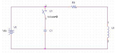
Figure1:An RLC circuit to charge and dischage a capacitor

The function is given as follows:
f(R)=e-Rt/2Lcos[√ (1/LC+ (R/2L)2t]-q/q0
In this section,we have to calculate the resistance in MATLAB using Newton-Raphson Method
MATLAB Files:

Name this function file as the RLC.m


function f_value=RLC(R);
t=0.05;
q0=5e-4;
q=5e-6;
L=5;
C=1e-4;
f_value=(exp(-R*t/(2*L)))*cos(sqrt((1/(L*C))-(R/(2*L))^2)*t)-q/q0;


Code derivative function of the given equation:
function f_valueD=RLC_D(R);
f_valueD=(R*t)/((4*L^2)*(sqrt(1/(L*C)-(R/(2*L))^2)))*(exp(-R*t/(2*L)))*sin(sqrt((1/(L*C))-(R/(2*L))^2)*t)-(t/(2*L))*(exp(-R*t/(2*L)))*cos(sqrt((1/(L*C))-(R/(2*L))^2)*t);

%code for Newton-Raphson(Main File):
clc;
clear all
tic
Ri=200;
es=0.0001;
j=0;
jmax=25;
while(1)
fi=RLC(Ri)
fid=RLC_D(Ri)
Ril=Ri-fi/fid
if Ril~=0
ea=abs((Ril-Ri)/Ril)*100
end
if ea=jmax
break
end
fp=fopen('iea.txt', 'a+');
[err, msg]=ferror(fp, 'clear');
if err~=0
disp('An error occurred while appending data to the file')'
disp(msg)
end
fprintf(fp, '%0.0f\t %8.5e\n',j,ea);
err=fclose(fp);
if err~=0
disp('could not close the file')
end
Ri=Ril
j=j+1
end
disp('The value of resistance is: ')
disp(Ril)
disp('The value of j is: ')
disp(j)
toc

Output:
fi =
-0.1631
fid =
0.0016
Ril =
301.8218
ea =
33.7357
Ri =
301.8218
j =
1
fi =
-0.0275
fid =
0.0011
Ril =
326.9259
ea =
7.6788
Ri =
326.9259
j =
2

fi =
-0.0012
fid =
9.9975e-004
Ril =
328.1487

ea =
0.3726
Ri =
328.1487
j =
3
fi =
-2.6963e-006
fid =
9.9534e-004
Ril =
328.1514
ea =
8.2550e-004
Ri =
328.1514
j =
4
fi =
-1.3185e-011
fid =
9.9533e-004
Ril =
328.1514
ea =
4.0369e-009
The value of resistance is:
328.1514
The value of j is:
4
elapsed_time =
0.0940


Result:

The value of resistance, R is = 328.1514

Conclusion:

We have already studied two methods those are close methods, i.e. they need two initial guesses. In this experiment, we study another method that is open method, i.e. it needs one initial guess. Here we learn the Newton-Raphson Method very clearly and clarify the process of writing the MATLAB code.

Download Link.exe(free)

In Microprocessors And Interfacing lab. we need a file called link.exe.This will help you to create a link to .obj.So download this file for free. DOWNLOAD LINK:
Download LINK.exe

How it works:

Run the file LINK.EXE with your created object file name after it
LINK.EXE EXP1.OBJ or
LINK EXP1
You will see:

c:\mda>link exp1
Microsoft (R) Overlay Linker Version 3.60
Microsoft Corp 1983‐1987. All rights reserved.
Run File [exp1.EXE]:

Download masm.exe(free)

In Microprocessors And Interfacing lab. we need a file called masm.exe.This will help you to complie the file that you have written already in .asm.Also tell you that if any errors happened in .asm.So download this file for free.

DOWNLOAD LINK: Download masm.exe


How it works:

Run the file MASM.EXE with your asm file name after it
MASM.EXE EXP1.ASM or
MASM EXP1

You will see

C:\mda>masm exp1
Microsoft (R) Macro Assembler Version 5.10
Copyright (C) Microsoft Corp 1981, 1988. All rights reserved.
filename [exp1.OBJ]

Press enter to create exp1.OBJ file then
Source listing [NUL.LST]: Press enter if list file is not needed
Press any name and enter if list file is needed

cross-correlation of two discrete sequence using conv in matlab

First we will find convolution of two discrete signals and then crosscorrelation of two signals using conv and xcorr function.
MATLAB Code:

clc;
a=[2 3 1];
b=[1 2 3];
c=conv(a,b);
m=length(c)-1;
n=0:1:m;
subplot(3,1,1);
stem(n,c);
xlabel('n');
ylabel('c');
title('convolution of two discrete sequence using conv function');
x=[1 2 3];
y=[1 2 3];
n1=length(y)-1;
n2=length(x)-1;
r1=conv(x,fliplr(y));
r=xcorr(x,y);
k=-n1:n2;
subplot(3,1,2);
stem(k,r);
xlabel('k');
ylabel('r');
title('cross-correlation of two discrete sequence using conv and xcorr function');
subplot(3,1,3);
stem(k,r1);


Output:

Checking Linearity of given signal

Checking Linearity of given signal,y(n)=nx(n)
Matlab Code
clc;
n=0:10;
a=2;
b=-3;
x1=cos(2*pi*.1*n);
x2=cos(2*pi*.5*n);
x=a.*x1+b.*x2;
y=n.*x;
y1=n.*x1;
y2=n.*x2;
yt=a.*y1+b.*y2;
d=y-yt;
subplot(3,1,1);
stem(n,y);
subplot(3,1,2);
stem(n,yt);
subplot(3,1,3);
stem(n,d);
axis([0 40 -10 20]);
Output:
Conclusion:A linear system is one that satisfies the superposition principles. Simply stated, the principle of superposition requires that the responses of the systems to a weighted sum of signal be equal to the corresponding weighted sum of the responses (outputs) of the systems to each of the individual input signals. Hence we have the following definition of linearity.Here from the figure1 we first plotted the linear combination of input and then plotted the linear combination of output and then plotted the difference.The difference between them is zero or equal.So the system is linear.

discreting an analog signal at different sampling rate


MATLAB Code:


f=10;
dt=.00005;
t=-.25:dt:.25;
xa=3*cos(2*pi*f*t);
subplot(5,1,1);
plot(t,xa); %plotting analog signal
xlabel('Time');
ylabel('Analog xa');
title('continuous time signal');
Ts=0.001; %sampling time .001
n=0:Ts:1;
xd=3*cos(2*pi*f*n);
k=0:(length(n)-1);
subplot(5,1,2);
stem(k,xd);
Ts=0.003; %sampling time .003
n=0:Ts:1;
xd=3*cos(2*pi*f*n);
k=0:(length(n)-1);
subplot(5,1,3);
stem(k,xd);
Ts=0.004; %sampling time .004
n=0:Ts:1;
xd=3*cos(2*pi*f*n);
k=0:(length(n)-1);
subplot(5,1,4);
stem(k,xd);
Ts=0.05; %sampling time .05
n=0:Ts:1;
xd=3*cos(2*pi*f*n);
k=0:(length(n)-1);
subplot(5,1,5);
stem(k,xd);


Output: