Finding root of an equation using Newton-Rapshon Method

Newton-Raphson Method, the most widely used of all root-locating formulas. If the function, f(x)
and an initial guess, xi is known then we can easily draw a tangent at the point [x_i, f(x_i)]. The

point where the tangent crosses the x-axis usually represents an improved estimate of the root.

The formula is derived geometrically from the straight line equation as the first derivative of the
function f(x) represents the slop of the tangent at that particular point.

A simple algorithm for the Newton-Raphson Method is given below:

1. Choose an initial guess that will be close to the true root.

2. An estimate of the root(ε_s) is determined by
x_i+1=x_i - f(x_i)/f’(x_i);
3. Evaluate the approximate percentage of errors(ε_a) by using the following formula:
ε_a= ((x_i+1- x_i)/ (x_i+1))*100%
If ε_a < ε_s, specified error tolerance, then stop the iteration; otherwise go to step 2. The process
is repeated until this condition is met.

In this experiment we will see how MATLAB can assist us in finding the roots of various functions using the numerical techniques Newton-Raphson method.


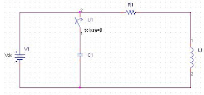
An experimental Circuit for the Newton raphson Method:

The circuit in Figure:1 charges the capacitor from the DC source when the switch is in its rest position.At t=0 sec,the is thrown at "2" position and the capacitor starts to discharge the RLC series circuit.



Figure1:An RLC circuit to charge and dischage a capacitor

The function is given as follows:
f(R)=e^-Rt/2Lcos[√ (1/LC+ (R/2L)²t]-q/q0
In this section,we have to calculate the resistance in MATLAB using Newton-Raphson Method
MATLAB Files:

Name this function file as the RLC.m

function f_value=RLC(R);
t=0.05;
q0=5e-4;
q=5e-6;
L=5;
C=1e-4;
f_value=(exp(-R*t/(2*L)))*cos(sqrt((1/(L*C))-(R/(2*L))^2)*t)-q/q0;

Code derivative function of the given equation:

function f_valueD=RLC_D(R);
f_valueD=(R*t)/((4*L^2)*(sqrt(1/(L*C)-(R/(2*L))^2)))*(exp(-R*t/(2*L)))*sin(sqrt((1/(L*C))-(R/(2*L))^2)*t)-(t/(2*L))*(exp(-R*t/(2*L)))*cos(sqrt((1/(L*C))-(R/(2*L))^2)*t);

%code for Newton-Raphson(Main File):

clc;
clear all
tic
Ri=200;
es=0.0001;
j=0;
jmax=25;
while(1)
fi=RLC(Ri)
fid=RLC_D(Ri)
Ril=Ri-fi/fid
if Ril~=0
ea=abs((Ril-Ri)/Ril)*100
end
if ea=jmax
break
end
fp=fopen('iea.txt', 'a+');
[err, msg]=ferror(fp, 'clear');
if err~=0
disp('An error occurred while appending data to the file')'
disp(msg)
end
fprintf(fp, '%0.0f\t %8.5e\n',j,ea);
err=fclose(fp);
if err~=0
disp('could not close the file')
end
Ri=Ril
j=j+1
end
disp('The value of resistance is: ')
disp(Ril)
disp('The value of j is: ')
disp(j)
toc

Output:

fi =
-0.1631
fid =
0.0016
Ril =
301.8218
ea =
33.7357
Ri =
301.8218
j =
1
fi =
-0.0275
fid =
0.0011
Ril =
326.9259
ea =
7.6788
Ri =
326.9259
j =
2

fi =
-0.0012
fid =
9.9975e-004
Ril =
328.1487

ea =
0.3726
Ri =
328.1487
j =
3
fi =
-2.6963e-006
fid =
9.9534e-004
Ril =
328.1514
ea =
8.2550e-004
Ri =
328.1514
j =
4
fi =
-1.3185e-011
fid =
9.9533e-004
Ril =
328.1514
ea =
4.0369e-009
The value of resistance is:
328.1514
The value of j is:
4
elapsed_time =
0.0940

Result:
The value of resistance, R is = 328.1514

Conclusion:
We have already studied two methods those are close methods, i.e. they need two initial guesses. In this experiment, we study another method that is open method, i.e. it needs one initial guess. Here we learn the Newton-Raphson Method very clearly and clarify the process of writing the MATLAB code.